── Conflicts ────────────────────────────────────────── tidyverse_conflicts() ──
✖ readr::col_factor() masks scales::col_factor()
✖ purrr::discard()    masks scales::discard()
✖ dplyr::filter()     masks stats::filter()
✖ dplyr::lag()        masks stats::lag()
ℹ Use the conflicted package (<http://conflicted.r-lib.org/>) to force all conflicts to become errors
read_csv("data/energy_data.csv")
Rows: 259 Columns: 10
── Column specification ────────────────────────────────────────────────────────
Delimiter: ","
chr (1): Country
dbl (9): electricity_access_percent, electricity_generating_capacity_kW, coa...

ℹ Use `spec()` to retrieve the full column specification for this data.
ℹ Specify the column types or set `show_col_types = FALSE` to quiet this message.
# A tibble: 259 × 10
Country electricity_access_p…¹ electricity_generati…² coal_metric_tons
<chr> <dbl> <dbl> <dbl>
1 AFGHANISTAN 97 776000 2096000
2 AKROTIRI NA NA NA
3 ALBANIA 100 2531000 9000
4 ALGERIA 99 21694000 0
5 AMERICAN SAMOA 59 47000 NA
6 ANDORRA 100 115837000 546000
7 ANGOLA 48 7344000 0
8 ANGUILLA 100 NA NA
9 ANTARCTICA NA 0 NA
10 ANTIGUA AND B… 100 117000 NA
# ℹ 249 more rows
# ℹ abbreviated names: ¹electricity_access_percent,
# ²electricity_generating_capacity_kW
# ℹ 6 more variables: petroleum_bbl_per_day <dbl>,
# refined_petroleum_products_bbl_per_day <dbl>,
# refined_petroleum_exports_bbl_per_day <dbl>,
# refined_petroleum_imports_bbl_per_day <dbl>, …
read_csv("data/demographics_data.csv")
Rows: 259 Columns: 14
── Column specification ────────────────────────────────────────────────────────
Delimiter: ","
chr (6): Country, Population_Growth_Rate, Total_Literacy_Rate, Male_Literacy...
dbl (7): Birth_Rate, Death_Rate, Net_Migration_Rate, Median_Age, Sex_Ratio, ...
num (1): Total_Population

ℹ Use `spec()` to retrieve the full column specification for this data.
ℹ Specify the column types or set `show_col_types = FALSE` to quiet this message.
# A tibble: 259 × 14
   Country         Total_Population Population_Growth_Rate Birth_Rate Death_Rate
   <chr>                      <dbl> <chr>                       <dbl>      <dbl>
 1 AFGHANISTAN             39232003 2.26%                       34.8       12.1
 2 AKROTIRI                      NA <NA>                        NA         NA
 3 ALBANIA                  3101621 0.19%                       12.5        7.36
 4 ALGERIA                 44758398 1.27%                       17.8        4.33
 5 AMERICAN SAMOA             44620 1.74%                       16.2        6.19
 6 ANDORRA                    85468 0.11%                        6.87       7.98
 7 ANGOLA                  35981281 3.34%                       41.4        7.8
 8 ANGUILLA                   19079 1.77%                       11.9        4.72
 9 ANTARCTICA                    NA <NA>                        NA         NA
10 ANTIGUA AND BA…           101489 1.13%                       15.0        5.69
# ℹ 249 more rows
# ℹ 9 more variables: Net_Migration_Rate <dbl>, Median_Age <dbl>,
#   Sex_Ratio <dbl>, Infant_Mortality_Rate <dbl>, Total_Fertility_Rate <dbl>,
#   Total_Literacy_Rate <chr>, Male_Literacy_Rate <chr>,
#   Female_Literacy_Rate <chr>, Youth_Unemployment_Rate <chr>
data_clean1 <-read_csv("data/dataclean1.csv")
New names:
Rows: 254 Columns: 10
── Column specification
──────────────────────────────────────────────────────── Delimiter: "," chr
(1): country dbl (9): ...1, electricity_generated_kw, coal_mt, nat_gas_cm,
co_emissions_m...
ℹ Use `spec()` to retrieve the full column specification for this data. ℹ
Specify the column types or set `show_col_types = FALSE` to quiet this message.
• `` -> `...1`
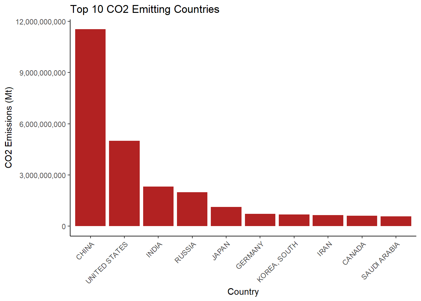
# A tibble: 10 × 2
   country       emissions_tons
   <chr>                  <dbl>
 1 CHINA            11535200000
 2 UNITED STATES     5006000000
 3 INDIA             2314738000
 4 RUSSIA            1985000000
 5 JAPAN             1135887000
 6 GERMANY            726881000
 7 KOREA, SOUTH       686000000
 8 IRAN               646000000
 9 CANADA             612000000
10 SAUDI ARABIA       579000000
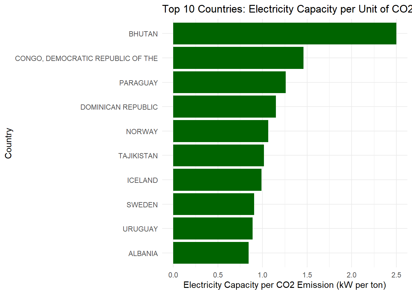
# A tibble: 10 × 2
   country                           capacity_per_emission
   <chr>                                             <dbl>
 1 BHUTAN                                            2.50
 2 CONGO, DEMOCRATIC REPUBLIC OF THE                 1.46
 3 PARAGUAY                                          1.26
 4 DOMINICAN REPUBLIC                                1.15
 5 NORWAY                                            1.07
 6 TAJIKISTAN                                        1.02
 7 ICELAND                                           0.989
 8 SWEDEN                                            0.906
 9 URUGUAY                                           0.891
10 ALBANIA                                           0.844
ggplot(top10_capacity_per_emission, aes(x = capacity_per_emission,y =reorder(country, capacity_per_emission))) +geom_col(fill ="darkgreen") +labs(title ="Top 10 Countries: Electricity Capacity per Unit of CO2 Emissions",x ="Electricity Capacity per CO2 Emission (kW per ton)",y ="Country" ) +theme_minimal()
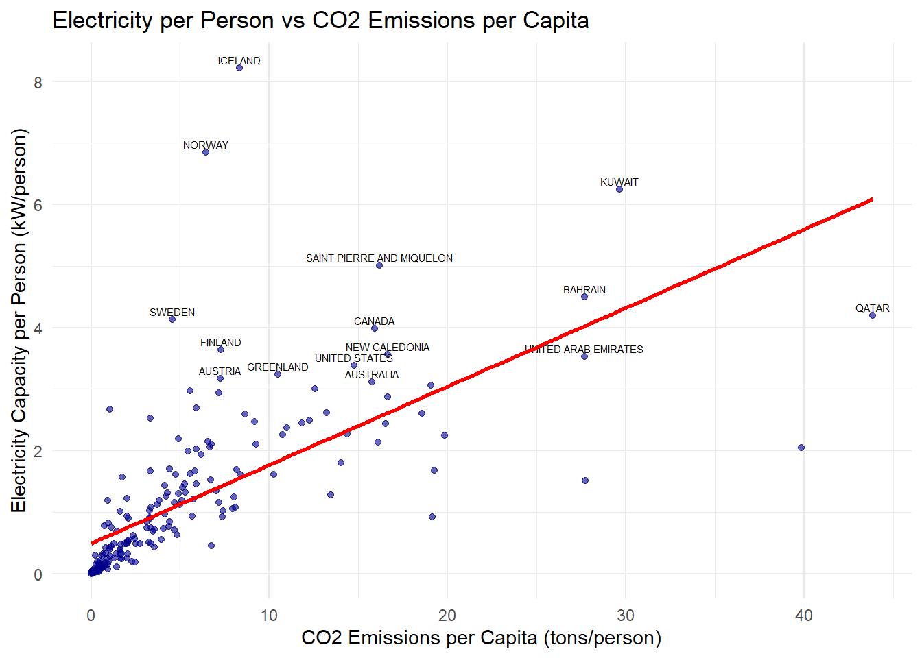
4. Which countries generate more electricity per person while keeping emissions per capita lower?
data_clean1 <- data_clean1 |>mutate(capacity_per_person = electricity_generated_kw / population)top10 <- data_clean1 |>arrange(desc(capacity_per_person)) |>head(n =15)ggplot(data_clean1, aes(x = emissions_per_capita, y = capacity_per_person)) +geom_point(alpha =0.6, color ="darkblue") +geom_text(data = top10, aes(label = country), vjust =-0.5, size =2) +geom_smooth(method ="lm", se =FALSE, color ="red") +labs(title ="Electricity per Person vs CO2 Emissions per Capita",x ="CO2 Emissions per Capita (tons/person)",y ="Electricity Capacity per Person (kW/person)" ) +theme_minimal()
`geom_smooth()` using formula = 'y ~ x'
Warning: Removed 57 rows containing non-finite outside the scale range
(`stat_smooth()`).
Warning: Removed 57 rows containing missing values or values outside the scale range
(`geom_point()`).
top10 |>select(country, capacity_per_person)
# A tibble: 15 × 2
   country                   capacity_per_person
   <chr>                                   <dbl>
 1 ICELAND                                  8.22
 2 NORWAY                                   6.85
 3 KUWAIT                                   6.24
 4 SAINT PIERRE AND MIQUELON                5.00
 5 BAHRAIN                                  4.49
 6 QATAR                                    4.20
 7 SWEDEN                                   4.13
 8 CANADA                                   3.98
 9 FINLAND                                  3.64
10 NEW CALEDONIA                            3.56
11 UNITED ARAB EMIRATES                     3.53
12 UNITED STATES                            3.38
13 GREENLAND                                3.24
14 AUSTRIA                                  3.17
15 AUSTRALIA                                3.12
Making a map
library(readr)library(rnaturalearth)
Warning: package 'rnaturalearth' was built under R version 4.5.2
library(rnaturalearthdata)
Warning: package 'rnaturalearthdata' was built under R version 4.5.2
Attaching package: 'rnaturalearthdata'
The following object is masked from 'package:rnaturalearth':

    countries110
library(sf)
Warning: package 'sf' was built under R version 4.5.2
Linking to GEOS 3.13.1, GDAL 3.11.4, PROJ 9.7.0; sf_use_s2() is TRUE
library(countrycode)
Warning: package 'countrycode' was built under R version 4.5.2
Warning: There was 1 warning in `mutate()`.
ℹ In argument: `iso3c = countrycode(country, "country.name", "iso3c")`.
Caused by warning:
! Some values were not matched unambiguously: AKROTIRI, ARCTIC OCEAN, ASHMORE AND CARTIER ISLANDS, ATLANTIC OCEAN, CLIPPERTON ISLAND, CORAL SEA ISLANDS, DHEKELIA, EUROPEAN UNION, INDIAN OCEAN, JAN MAYEN, KOSOVO, NAVASSA ISLAND, PACIFIC OCEAN, PARACEL ISLANDS, SAINT MARTIN, SOUTHERN OCEAN, SPRATLY ISLANDS, VIRGIN ISLANDS, WAKE ISLAND, WORLD
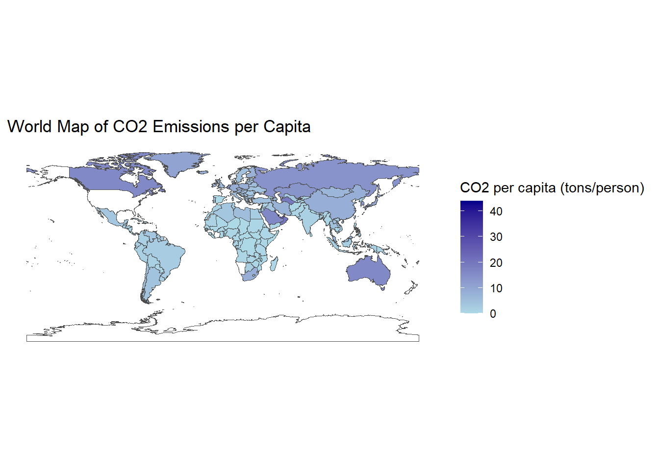
world <-ne_countries(scale ="medium", returnclass ="sf") %>%mutate(iso3c = iso_a3)world_emissions <- world |>left_join(data_map, by ="iso3c")ggplot(world_emissions) +geom_sf(aes(fill = emissions_per_capita), color ="gray30", size =0.1) +scale_fill_gradient(name ="CO2 per capita (tons/person)",low ="lightblue",high ="darkblue",na.value ="white" ) +labs(title ="World Map of CO2 Emissions per Capita") +theme_classic()